1. What are recommendation and retrieval tasks?
1.1 Examples from industry
Both recommender systems and retrieval systems aim to provide users with personalized rankings of items from a large catalog. The main difference between the two lies in the nature of the query: recommender systems typically generate recommendations that implicitly reflect user preferences based on their history and context, while retrieval systems often respond to explicit user queries. Many large-scale systems in industry implement both recommendation and retrieval functionalities: on any e-commerce platform, users can both search for specific products (retrieval) and receive personalized product suggestions based on their browsing and purchase history (recommendation).
From a technical standpoint, both types of systems share similar architectures and challenges, such as handling large catalogs, ensuring low latency, and providing relevant results. They mostly differ from the way to encode the (implicit vs explicit) query and from potentially using different evaluation metrics, but are otherwise quite similar. The following table summarizes some well-known systems in industry, as well as key quantities that drive the design of recommender & retrieval systems: their catalog sizes, typical query latencies, and the number of recommendations they have to generate per second.
| Reco/Retrieval System | Catalog size | Query latency | Reco per seconds |
|---|---|---|---|
| Google (search) | ~400B documents | < 200 ms | hundreds of thousands |
| Amazon | ~600M products | < 200 ms | tens of thousands |
| Netflix | ~5k movies & shows | minutes1 | thousands |
| Spotify | ~100M songs | minutes2 | (tens of) thousands |
| Criteo (advertising) | ~15B products | < 20 ms | hundreds of thousands |
At high level, both recommender systems and retrieval systems can be summarized as follows: the user has an history of events that are collected by the system, such as page views, clicks, purchases, ratings, ads, previous recommendations, and optionally an explicit query. Based on this information, the system has to look into a large catalog of items and produce a personalized ranking of the most relevant items to show to the user. The user then provides some feedback based on the ranking displayed, such as clicks, watch time, purchases, ratings, etc, that feeds the history of the user for future recommendations.
1.2 Formalization of the task
The query. All the information available about the query is summarized in a context variable \(x\) that belongs to some space \(\mathcal{X}\). The context \(x\) can contain a lot of different information depending on the application. Typically, it can contain the whole history of interactions of a user with the system, his profile information, the time of the day, the device used, the text of the query if there is one, etc.
The ranking. A recommender or retrieval system can be represented as a ranking function that, given a user context \(x\in\mathcal{X}\), outputs a top-\(k\) ranking over the catalog of \(n\) items. The set of outputs is then \(\mathfrak{S}^k_n\), the set of top-\(k\) permutations of \(n\) items.
\[\begin{align} \mathfrak{S}^k_n = \{\sigma : \{1, \ldots, k\}\to\{1, \ldots, n\} ~|~ \sigma ~~\text{is injective}\} \end{align}\]The injectivity constraint simply reflects the fact that an item cannot appear twice in the same ranking. However, manipulating top-\(k\) permutations is mathematically cumbersome and leads to overly complicated notations, so for all formalizations, we will consider that the output is a full ranking (a permutation) of the \(n\) items, even though, practically, only the top-\(k\) items matter and the \((n-k)\) last items could be in any order. In the end,
\[\begin{align} \text{Output space:}~~~\mathfrak{S}_n = \{\sigma : \{1, \ldots, n\}\to\{1, \ldots, n\} ~|~ \sigma ~~\text{is bijective}\} \end{align}\]Because permutations are always a bit tricky to remember, I encourage you to have a note in a corner: for a rank \(r\), I’ll stick with the notation that \(i = \sigma(r)\) is the item \(i\) at rank \(r\), and \(\sigma^{-1}(i) = r\) is the rank \(r\) of item \(i\).
The ranking function. At its core, a recommender system is a function \(h : \mathcal{X} \to \mathfrak{S}_n\) that maps contexts to rankings. There is a lot of literature on the class of function \(\mathcal{H} \subseteq \left(\mathcal{X} \to \mathfrak{S}_n\right)\) to use – i.e. the architecture of the recommender system. The important questions about this design choice relate to scalability, sequential modeling, latency constraints, etc. This will be developed in Section 2.
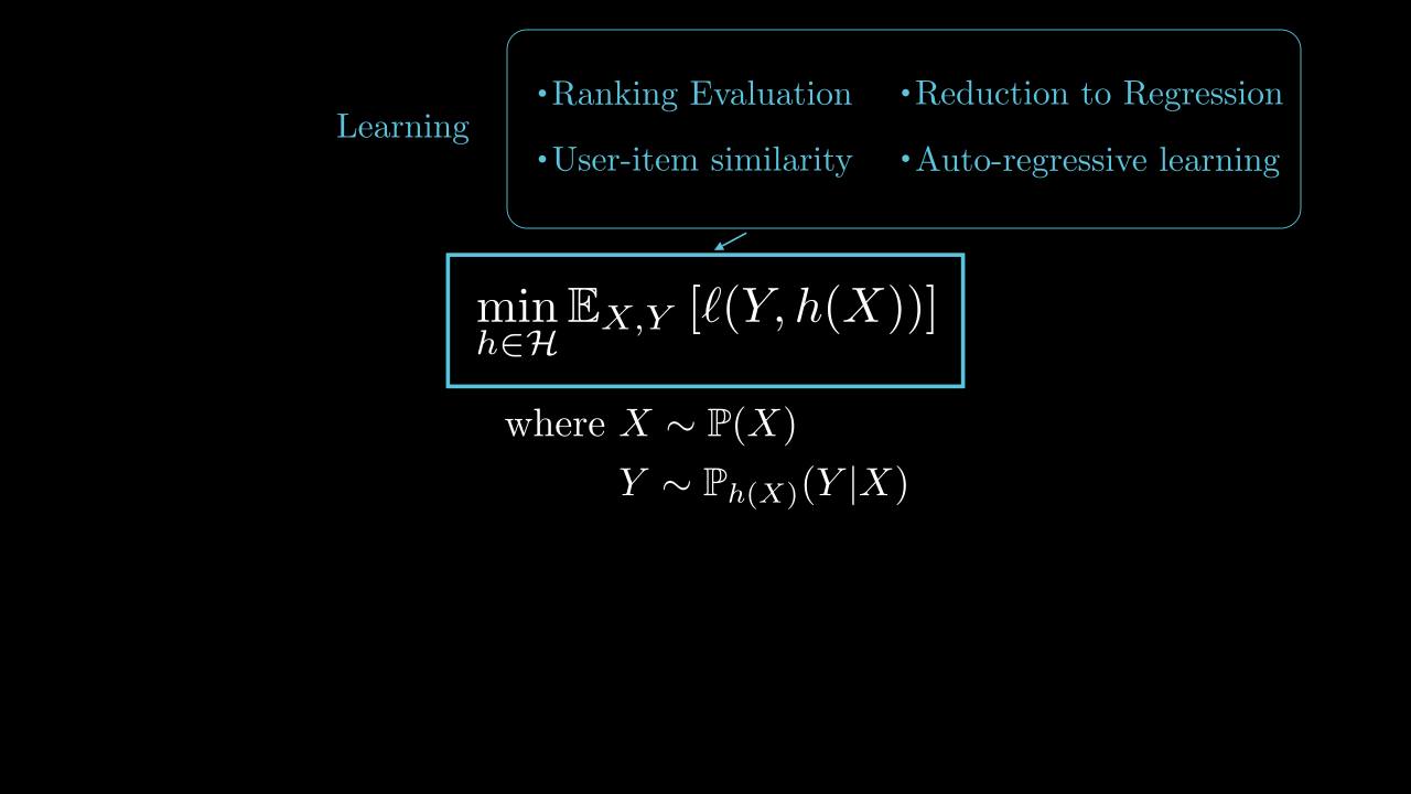
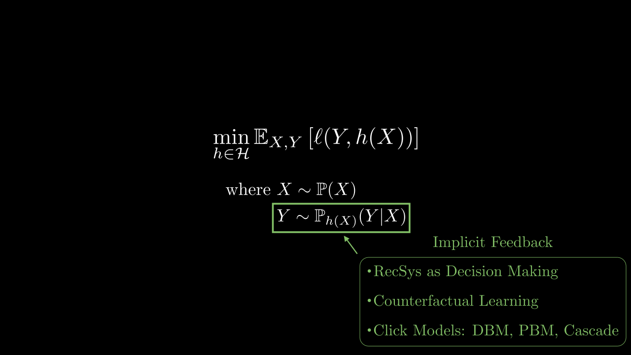
The feedback. Given a query context \(x\) and a ranking \(\sigma \in \mathfrak{S}_n\), the user provides some feedback \(y\) that belongs to some space \(\mathcal{Y}\). The feedback can take many different forms depending on the application. It can be explicit feedback like ratings, or implicit feedback like clicks, watch time, purchases, etc. Unfortunately, in many applications, the feedback is implicit, which means that, as a random variable, the feedback \(Y\) not only depends on the context \(X\) but also on the ranking \(\Sigma\) displayed to the user.
Learning the ranking function. Finally, the ranking function \(h\in\mathcal{H}\) needs to be learned from data collected over time. This data consists of triplets \((X, \Sigma, Y)\), where \(X\) is the context, \(\Sigma\) the ranking displayed to the user and \(Y\) the feedback provided by the user. Depending on whether the feedback is implicit (\(Y \not\mathrel{\perp\!\!\!\!\perp}\Sigma | X\)) or explicit (\(Y \mathrel{\perp\!\!\!\!\perp}\Sigma | X\)), the learning problem differs. The objective is to minimize a loss \(\ell\) (or eq. maximize a reward). For explicit feedback, classical supervised learning techniques with losses and metrics adapted to the ranking setting can be used (Section 3). For implicit feedback, the learning task is more complex and related to the (combinatorial) bandit setting (Section 4). The following picture summarizes the main components of a recommender system and the organization of this course.
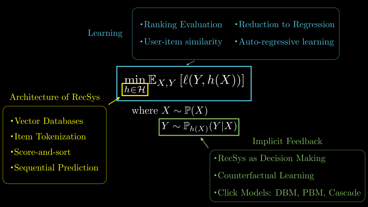
Section 2 details the different architectural choices that can be made to build a recommender system, emphasizing the challenges related to scalability and combinatorial prediction. Section 3 focuses on the supervised learning setting, where the feedback is explicit and does not depend on the ranking displayed to the user, digging into learning to rank and sequential modeling for user histories. Finally, Section 4 focuses on the implicit feedback setting, where the feedback depends on the ranking displayed to the user, and details bandit algorithms for recommender systems.
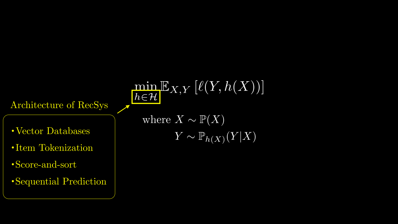
2. Architecture for large-scale recommender systems
As a reminder, this section focuses on the architecture of the recommender system – i.e. the class of function \(\mathcal{H}\) chosen to build a recommendation given all know inputs.
Recommender systems have several key challenges that influence their architecture.
Scalability of inference. Recommender systems often need to handle a very large number of items. The number of items \(n\) is particularly challenging, as each time the system needs to produce a ranking, it potentially has to consider all the items. However, for many applications, an inference time of \(O(n)\) is not acceptable, as \(n\) can be in the millions or even billions (e.g. online retail platforms). Two main approaches have been developed to tackle this scalability issue.
- Vector DB based: The system is broken down in two steps. A first step leverages a Vector Database to index item embeddings for fast retrieval (Section 2.1.1), and is followed by a re-ranking step with more complex models, but that only considers the subset of retrieved items.
- Token-based: Similarly to text-related models, the system encodes items as a sequence or a vector of tokens, where the number of tokens is much smaller than the number of items. Then the prediction function predicts sequences of tokens instead of directly predicting items (Section 2.1.2).
Combinatorial aspect of the prediction. The output space of the recommender system is combinatorial in nature, as it consists of rankings over a large number of items. There are different ways to build such a prediction function and two approaches are detailed in the following sections.
- Score-and-sort. The recommender system first computes a vector of scores (one for each items or tokens) and then sorts the items according to their scores to produce a ranking (Section 2.2.1). This approach is simple and efficient, as it reduces the problem to predicting \(n\) scores (like classification), but does not allow to easily model interactions between items in the ranking.
- Sequential prediction. The recommender system builds the ranking sequentially, by predicting the first item (or token), then the second given the first, and so on, up to rank generating \(k\) items (Section 2.2.2). This approach allows to model interactions between items in the ranking, but is more complex and computationally expensive.3
Sequential modeling of the context. The context \(x\) represents all the information available about the user at the time of the query. In particular, it can contain the history of interactions of the user with the system. This history is often sequential in nature, as the order (and the time) of interactions matters. For instance, the last items viewed by a user are often more relevant than the ones viewed a long time ago. Therefore, the architecture of the recommender system needs to be able to model sequential data effectively, for instance using recurrent neural networks or transformers.
2.1 Scalability choices
2.1.1 Vector Database
The approach that has been adopted by most large-scale recommender systems is to break down the recommendation task into two steps:
- Vector DB step. Given a context \(x\), retrieve a small subset of relevant items from the large catalog of \(n\) items in time \(o(n)\). The goal is to reduce the complexity from \(n\) to a manageable number \(m\) (ex: \(m=1000\)).
- Re-ranking step. Given the context \(x\) and the \(m\) retrieved items, re-rank them using a more complex model that can take into account more features and interactions between items and users.
Vector databases rely on approximate nearest neighbor (ANN) search, or maximum inner product search (MIPS), to quickly find similar items in high-dimensional spaces. Locality Sensitive Hashing (LSH) is a vanilla ANN algorithm that illustrates the basic principles of how ANN works.
2.1.1.1 The Approximate Nearest Neighbor Problem
Given a set \(\mathcal{Z}\) of \(n\) vectors \(z_1,\dots, z_n \in \mathbb{R}^d~\) in a \(d\)-dimensional space and a query \(q\in \mathbb{R}^d\), the goal is to find the vector that is closest to the query. \[ \arg\max_{z_i \in \mathcal{Z}} \|q - z_i\|_2 \] This problem can be computationally expensive when the number of points is very large, which is often the case in real-world recommender systems for instance. The brute-force approach (🎥) is to compute the distance between the query and each point in the dataset, which means a retrieval time of \(O(n)\) for each query.
The difference between Approximate Nearest Neighbor (ANN) search and Maximum Inner Product Search (MIPS) is in the similarity measure used to compare vectors. ANN typically refers to the use of distance metrics like Euclidean distance, while MIPS refers to maximizing the inner product with the query vector. If the vectors are normalized, both problems are equivalent.
2.1.1.2 Locality Sensitive Hashing
Locality Sensitive Hashing (LSH) is the vanilla technique that allows to index vectors by hashing them in such a way that similar points are more likely to be hashed to the same index. The idea is to use a family of hash functions that are locality sensitive, meaning that they preserve the locality between points in some way.
This allows to reduce the retrieval time to be sublinear in \(n\), i.e. \(O(n^{\rho})\) for some \(0 <\rho < 1\). However, this comes at several costs.
- The algorithm is approximate, meaning that it may not always return the exact nearest neighbor. Given a query \(q\) and a given distance \(r>0\), LSH looks for a vector \(z_i\) such that \(\|q - z_i\|_2 \leq r\)
- With some controlled probability, the algorithm may fail to retrieve an approximate nearest neighbor.
- The algorithm requires a preprocessing step to build the hash table, which can be expensive in terms of time and space.
Hashing
The first step in LSH is to create a hash function that maps \(z_1,\dots, z_n\) to discrete hash codes. To do so, it relies on sampling \(k\) random hyperplanes (🎥).
Each hyperplane is defined by a normal vector \(\theta \in \mathbb{R}^d\) and a bias \(c \in \mathbb{R}\). An hyperplane divides the space into two half-spaces. Finding out on which side of hyperplane \(\theta\) a point \(z\) lies boils dow to checking
\[ H(z) ~~=~~ {\rm sign}(\theta^T z + c) \]
For each point of the database \(z_i\), the comparison with each of the \(k\) hyperplanes yields one bit. These bits are concatenated to form a \(k\)-bit hash code (🎥). All the vectors of the database are then stored in a hash table, where the key is the hash code. As several vectors can have the same hash code, each element of the hash table is a list, sometimes called a bucket.
Proposition 1 The preprocessing time is \(O(dkn)\) and the storage space is \(O(dn + dk + n)\).
\(~\)
Retrieval
Given a query \(q\), the same process is applied to compute its hash code. The hash table is then searched for the corresponding bucket (🎥). The query \(q\) is compared to vectors in the bucket up until finding an approximate nearest neighbor – i.e. vector \(z_i\) such that \(\|q - z_i\|_2 \leq r\).
To compute the complexity of the retrieval step and the success probability, we need two probabilities \(\alpha\) and \(\beta\) that characterize the family of method used to build the hash codes (here the hyperplanes).
Definition 1 (LSH Family) A family of hash functions is said to be \((r, cr, \alpha, \beta)\)-locality sensitive if it satisfies the following properties:
- Precision: Two points \(z_1, z_2\) “close enough” have a high probability of being hashed to the same bucket – i.e. \(\mathbb{P}_{H}\Big(H(z_1) = H(z_2) \Big| \|z_1 - z_2\|_2 \leq r\Big) \geq \alpha\)
- Recall: Two points \(z_1, z_2\) “far enough” have a low probability of being hashed to the same bucket – i.e. \(\mathbb{P}_{H}\Big(H(z_1) = H(z_2) \Big| \|z_1 - z_2\|_2 > cr\Big) \leq \beta\)
Here, we are using hyperplanes to illustrate the LSH algorithm. However, LSH can be used in the very same way with other families of hash functions, as long as they satisfy this property of being \((r, cr, \alpha, \beta)\)-locality sensitive. For instance, the MinHash family of hash functions is also locality sensitive. It is used to compute the Jaccard similarity between sets. The same principles apply, but the details of the algorithm are different.
Proposition 2 The retrieval time is at most \(O(dk + dn\beta^k)\) and the probability of success is at least \(\alpha^k\).
As the objective is to minimize the retrieval time, we would like to choose \(k \simeq \log(n)\), to obtain a complexity of \(O(d\log(n) + dn\beta^{\log(n)}) = O(d\log(n) + dn n^{\log(\beta)})\) that is sublinear in \(n\) as \(\log(\beta)<0\). Unfortunately, this would make the probability of success \(\alpha^{\log(n)}\) very small.
Multiple Hash Tables
The solution to circumvent the problem explained in the above remark is to use multiple hash tables (🎥), namely \(\tau\) of them. Indeed, the algorithm would only fail if it does not find an approximate nearest neighbor in any of the \(\tau\) hash tables. In the end, the complete LSH algorithms is tuned as follows:
Proposition 3 By choosing \(k = {{\log(n)} \over {-\log(\beta)}}\), \(\rho = {\log(\alpha) \over \log(\beta)}\) and \(\tau = n^{\rho}\), we have
- The retrieval time is \(O(dn^{\rho})\),
- The probability of success is at least \(1 - (1-n^{-\rho})^{n^\rho}\),
- The storage space is \(O(dn + n^{1+\rho})\),
- The preprocessing time is \(O(dn^{1+\rho}\log(n))\).
It may not be directly clear to you that \(\rho \in (0,1)\). It comes from the fact that two points that are “close enough” have a higher probability of being hashed to the same bucket than two points that are “far from each other”. Otherwise said, \(\alpha > \beta\), which in turns implies that \(\rho = {\log(\alpha) \over \log(\beta)} < 1\).
2.1.2 Item tokenization
With the success of large language models (LLMs) in natural language processing, another approach to build scalable recommender systems has emerged: item tokenization. The idea is to represent each item in the catalog as a sequence of tokens, similar to how words are represented in text processing. This allows to build models that predict sequences of tokens instead of directly predicting items, reducing the output space from \(n\) items to a much smaller vocabulary of \(v\) tokens.
Formally, the idea is to define a mapping from items to sequences of tokens: \[\begin{align} T : \{1, \ldots, n\} &\to \{1, \ldots, v\}^L \\ i &\mapsto (t_{i,1}, t_{i,2}, \ldots, t_{i,L}) \end{align}\] where \(L\) is the length of the token sequence and \(v\) is the size of the token vocabulary. Ideally, \(T\) would be invertible and the prediction function \(h : \mathcal{X}\to \mathfrak{S}_n\) would then be decomposed into two steps:
\[\begin{align} h ~~:~~ \mathcal{X}~~ \xrightarrow{~~~g~~~} ~~ \{1, \ldots, v\}^{L\times k} ~~ \xrightarrow{T^{-1}} ~~ \mathfrak{S}^k_n \end{align}\]
where \(g : \mathcal{X}\to \{1, \ldots, v\}^{L\times k}\) predicts a sequence of \(Lk\) tokens, corresponding to the \(k\) items in the ranking (using any sequence to-sequence model, such as transformers), and \(T^{-1}\) maps the predicted token sequences back to items.
However, practically, \(T\) is usually not invertible, simply because \(n\) is not necessarily decomposable as \(v^L\). The problem of non-surjectivity of \(T\) corresponds to hallucinations, where the model \(g\) predicts token sequences that do not correspond to any item in the catalog. The problem of non-injectivity of \(T\) corresponds to collisions, where multiple items are mapped to the same token sequence.
- Collisions can be handled by adding a re-ranking step after \(T^{-1}\) to choose the best item among the colliding ones.
- Hallucinations can be handled by constraining the decoding of \(g\) to only produce valid token sequences (e.g. beam search).
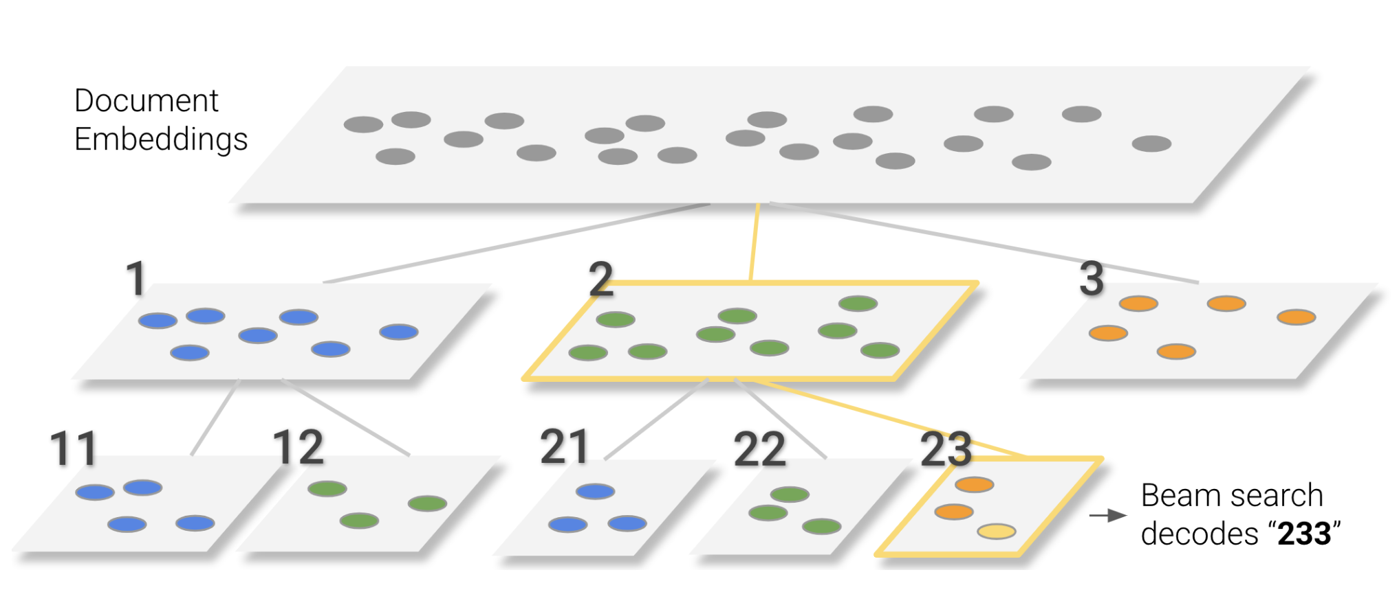
2.1.2.1 Hierarchical clustering
A quite intuitive way to build such a tokenization, that has been used in Tay et al. (2022), is to use hierarchical clustering on item embeddings. The idea is to build a hierarchical clustering tree over the item embeddings, where each node in the tree corresponds to a token.
Such a hierarchical clustering can be obtained by using any clustering algorithm recursively, such as k-means.
The path from the root to a leaf node (item) then defines the sequence of tokens representing that item. A clustering like this can simply be obtained by using k-means recursively to build a balanced tree of depth \(L\) with \(v\) clusters at each level.
2.1.2.2 RQ-VAE
The most popular idea nowadays is to learn item tokenization is to use a Residual Quantized Variational Autoencoder (RQ-VAE) as proposed in Rajput et al. (2023). The idea is to learn discrete item tokens by training a RQ-VAE to reconstruct item embeddings coming from a pre-trained model (e.g. TIGER architecture). It can also include additional losses such as a contrastive loss on the reconstruction of the item-item similarity matrix (Lepage, Mary, and Picard (2025)). I believe the schema from the original paper is better than a lengthy explanation, so here it is:
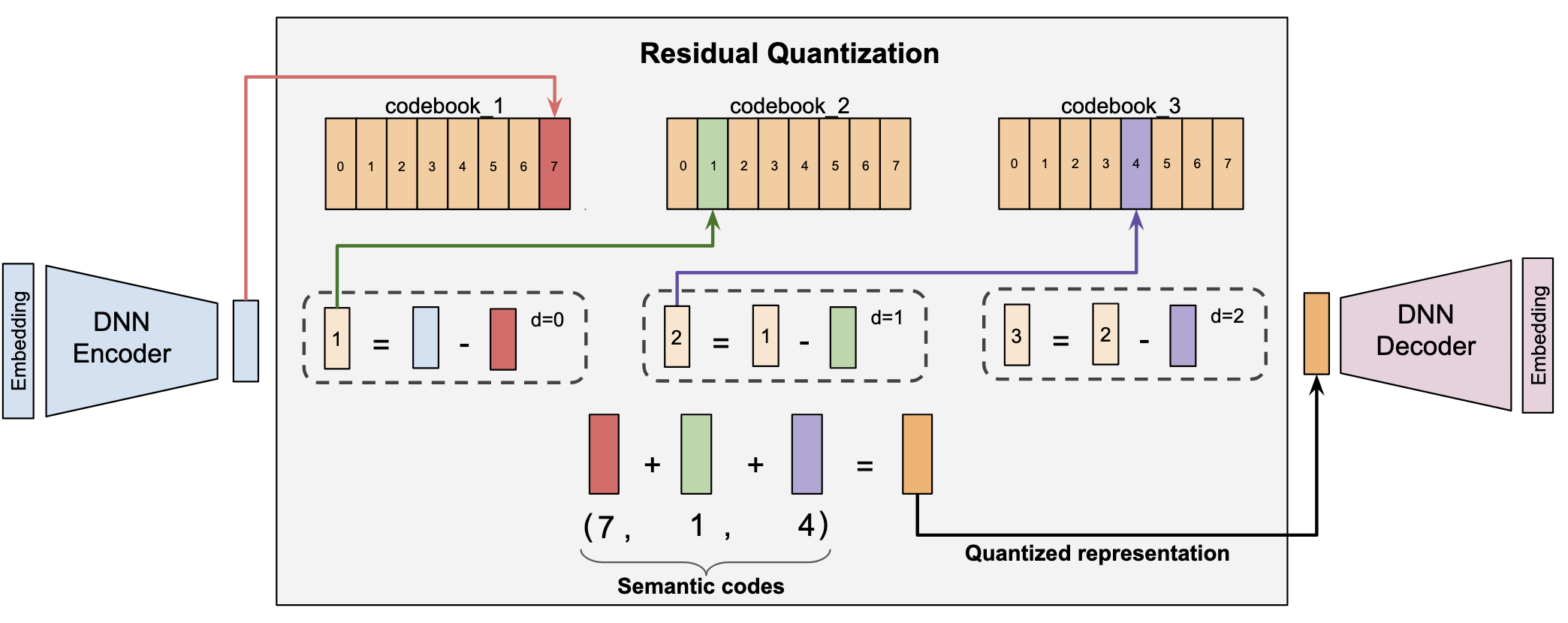
The item embedding is encoded using a RQ-VAE encoder into \(L\) discrete tokens, each token being selected from a codebook of size \(v\). The first token is selected by finding the token with closest embeddings to the item in the first codebook. Then, the residual between the item embedding and the embedding of the first token is computed, and the second token is selected by finding the closest token in the second codebook to this residual. This process is repeated \(L\) times to obtain a sequence of \(L\) tokens representing the item. The decoder part is only used during training to use a reconstruction loss between the original item embedding and the reconstructed embedding from the tokens.
2.2 Combinatorial prediction choices
2.2.1 Score-and-sort prediction
A common way to implement a prediction function \(h\) from \(\mathcal{X}\) to \(\mathfrak{S}_n\) is to decompose it in two-steps. First, a scoring function \(f:\mathcal{X}\to\mathbb{R}^n\) predicts one score per item. We denote \(\mathcal{F}\) a space of measurable functions from \(\mathcal{X}\) to \(\mathbb{R}^n\). This vector of scores \(s\in\mathbb{R}^n\) is mapped to \(\mathfrak{S}_n\) using the \(\mathop{\mathrm{argsort}}\) function to get a ranking. \[\begin{align} \mathop{\mathrm{argsort}}(s) = \left\{\sigma\in\mathfrak{S}_n: \forall r<n, s_{\sigma(r)} \geq s_{\sigma(r+1)}\right\} \end{align}\]
In the end, we have \[\begin{align} h ~~:~~ \mathcal{X}~~ \xrightarrow{~~~f~~~} ~~ \mathbb{R}^n ~~ \xrightarrow{\mathop{\mathrm{argsort}}} ~~ \mathfrak{S}_n \end{align}\]
An advantage of this approach is that it reduces the combinatorial prediction problem to a simpler prediction problem in \(\mathbb{R}^n\). Indeed, instead of learning \(h\) by minimizing some task loss, we can learn \(f\) by minimizing a surrogate loss (see Section 3.2).
Score and sort/select is not a restriction a priori: \(\mathcal{H}= \mathop{\mathrm{argsort}}\circ \mathcal{F}\). However, while \(\mathop{\mathrm{argsort}}\) is computable in \(\mathcal{O}(n\log(n))\) time, depending on the task at hand, the optimal prediction function \(f^*\) may have arbitrarily bad properties, such as being discontinuous (Calauzenes and Usunier (2020)). This is a problem as we would like the optimal predictor to be approximable by usual hypothesis classes, such as neural networks of finite size, SVMs…
2.2.2 Sequential prediction
Another way to build a prediction function \(h\) from \(\mathcal{X}\) to \(\mathfrak{S}_n\) is to decompose the ranking generation as a sequential prediction problem. The idea is to predict the ranking one item at a time, by predicting the item at rank 1, then the item at rank 2 given the first item, and so on, up to rank \(k\) (as a reminder, we only care about the \(k\) top items). Formally, in such case, the prediction function \(h\) is not a function anymore but a randomized predictor.
Formally, this can be done using the chain rule of probability to decompose the prediction of a ranking \(\sigma\) as a product of conditional probabilities: \[\begin{align} \mathbb{P}(\sigma | x) = \prod_{r=1}^k \mathbb{P}\left(\sigma(r) \middle| x, \sigma(1), \ldots, \sigma(r-1)\right) \end{align}\]
As it turns out, this decomposition corresponds to the way sequence-to-sequence models are trained in natural language processing. Therefore, we can leverage architectures such as transformers or recurrent neural networks to build such sequential prediction functions.
In order to accomodate the different levels of dependencies, such as “dependence on items from the same recommendation” vs “dependence on user history”, or such as “dependence between tokens within an item” vs “dependence between items”, different levels of sequential modeling can be used (e.g. Lepage, Mary, and Picard (2025) marius).
3. Learning to rank
In this chapter, we focus on learning the ranking function \(h \in \mathcal{H}\) from supervised data. This is a strong assumption, as in many applications, the feedback is implicit and depends on the ranking displayed to the user. However, this supervised setting is used either when the dependency of the feedback on the ranking is negligible enough (almost explicit feedback) or for pre-training the ranking function before fine-tuning it in an implicit feedback setting.
As a reminder, a learner has access to input features \(x\in\mathcal{X}\subseteq \mathbb{R}^{d}\)4 and wants to predict a permutation over \(n\) items formalized by a permutation \(\sigma\in\mathfrak{S}_n\). To do so, she needs to learn a prediction function \(h : \mathcal{X}\to \mathfrak{S}_n\), belonging to a space of measurable functions from \(\mathcal{X}\) to \(\mathfrak{S}_n\) denoted \(\mathcal{H}\), using some feedback \(y\in\mathcal{Y}\) and minimizing a task loss \(L: \mathcal{Y}\times \mathfrak{S}_n \to \mathbb{R}^+\) in expectation over some joint distribution \(p_{X,Y}\in\mathcal{D}\) on the observable variables:
\[\begin{align} \inf_{h\in\mathcal{H}} \mathcal{L}(p_{X,Y}, h)~~~~~~~~ \text{where}~~\mathcal{L}(p_{X,Y}, h) = \mathbb{E}_{p_{X,Y}}\left[\ell(Y, h(X))\right] \end{align}\]
3.1 Task Loss
Like in other supervised learning settings, the choice of the task loss \(\ell\) is crucial, as it defines what is a good prediction. For instance, in classification, typical task losses are the classification error (0/1 loss) or F1-score. In ranking, there is a wide variety of task losses that have been proposed in the literature, depending on the application and the type of feedback available. Popular examples are provided in Table 1.
| \(\mathcal{Y}\) | Loss | Formula |
|---|---|---|
| \(y\in\{0,\dots,p\}^n\) | \({\tt DCG@k}\) | \(- \sum\limits_{r=1}^k \frac{2^{y_{\sigma(r)}}-1}{\log(1+r)}\) |
| \({\tt NDCG@k}\) | \(\frac{-{\tt DCG@k}(y, \sigma)}{\max\limits_{\nu\in\mathfrak{S}_n}{\tt DCG@k}(y, \nu)}\) | |
| \({\tt ERR}\) | \(\substack{-\sum\limits_{r=1}^n \frac{R_{\sigma(r)}}{r} \prod\limits_{k=1}^{r-1}(1-R_{\sigma(k)})\\R_i = \frac{2^i-1}{2^p}}\) | |
| \(y\in\{0,1\}^n\) | \({{\tt Prec@k}}\) | \(-\sum\limits_{r=1}^k \frac{y_{\sigma(r)}}{k}\) |
| \({\tt Rec@k}\) | \(-\sum\limits_{r=1}^k \frac{y_{\sigma(r)}}{\lVert y\rVert_1}\) | |
| \({\tt AP}\) | \(\frac{-1}{\lVert y\rVert_1} \sum\limits_{i:y_i=1} {\tt Prec@\sigma^{-1}(i)(y, \sigma)}\) | |
| \({\tt MRR}\) | \(\frac{-1}{\lVert y\rVert_1} \sum\limits_{i:y_i=1} \frac{1}{\sigma^{-1}(i)}\) | |
| \({\tt AUC}\) | \(\sum\limits_{\substack{i:y_i=1\\j:y_j=0}}\frac{{\mathbb{I}_{\left[\sigma^{-1}(i) > \sigma^{-1}(j)\right]}}}{\lVert y\rVert_1(n-\lVert y\rVert_1)}\) | |
| \(y\in \text{DAG}_n\) | \({\tt PD}\) | \(\sum\limits_{i\to j \in y}{\mathbb{I}_{\left[\sigma^{-1}(i) > \sigma^{-1}(j)\right]}}\) |
| \(y\in\mathfrak{S}_n\) | \({\tt Spearman}\) | \(\frac{6}{n(n^2-1)}\sum\limits_{i=1}^n (\sigma^{-1}(i) - y^{-1}(i))^2 - 1\) |
| \({\tt K_\tau}\) | \(1-\frac{2}{n(n-1)}\sum\limits_{i,j=1}^n {\mathbb{I}_{\left[y^{-1}(i) < y^{-1}(j)\right]}}{\mathbb{I}_{\left[\sigma^{-1}(i) > \sigma^{-1}(j)\right]}}\) | |
| \({\tt ZO}\) | \(-{\mathbb{I}_{\left[\sigma = y\right]}}\) |
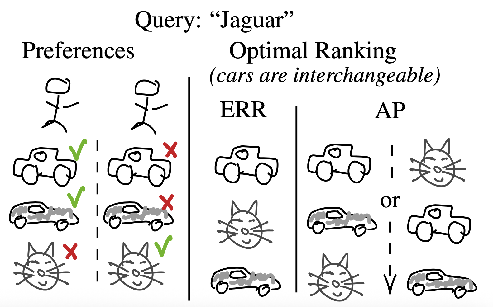
However, not all task losses are equally easy to optimize. For instance, \({\tt PD}\) is known to be NP-hard to optimize in general (Duchi, Mackey, and Jordan (2010)) and \({\tt ERR}\) and \({\tt AP}\) are known to be incompatibles with expected utilities (no simple reduction to regression) (Calauzènes, Usunier, and Gallinari (2012)).
The Expected Reciprocal Rank (\({\tt ERR}\)) task loss encourages diversity in the rankings it generates. This is due to its “winner-takes-all” nature, which stems from its cascade structure: the first relevant item found receives the majority of the credit, while subsequent relevant items contribute significantly less. Consequently, for queries with multiple intents, the model is incentivized to prioritize items relevant to different intents before selecting additional items relevant to the same intent. On the other side of the spectrum, the \({\tt AP}\) is diversity-averse (see example below)
Both Spearman’s rank correlation (\({\tt Spearman}\)) and Kendall’s tau (\({\tt K_\tau}\)) are metrics (in the mathematical sense) on the space of permutations. In fact, \({\tt Spearman}\) can simply be seen as the Pearson correlation coefficient between the rank vectors of two permutations.
The learning method largely depends on the nature of the feedback observed \(\mathcal{Y}\). For instance, if the feedback is a relevance score (e.g. ratings), the learner can use regression techniques to predict these scores and then use them to generate a ranking. If the feedback is a binary preference feedback (e.g. whether item \(A\) is preferred over item \(B\)), the learner will have to turn towards pairwise learning to rank methods… These are developed in the next sections.
3.2 Score-and-sort learning approaches
As explained in Section 2.2.1, a common way to build a ranking function \(h\) is to decompose \(\mathcal{H}= \mathop{\mathrm{argsort}}\circ \mathcal{F}\), where \(\mathcal{F}\) is a subset of the space of measurable functions from \(\mathcal{X}\) to \(\mathbb{R}^n\).
However, because of the non-continuity introduced by the \(\mathop{\mathrm{argsort}}\) function, directly minimizing the task loss \(\ell\) over \(h\in\mathcal{H}\) is generally intractable, even for “well-behaved” choices for \(\mathcal{F}\), such as neural networks.
For this reason, \(f\) is usually learnt using a more convenient (e.g. continuous or even convex) surrogate loss \(\phi: \mathcal{Y}\times \mathbb{R}^m \to \mathbb{R}^+\) by solving:
\[ \inf_{f\in\mathcal{F}} \Phi(p_{X,Y}, f)~~~~~~~~~~~~ \text{where}~~\Phi(p_{X,Y}, f) = \mathbb{E}_{p_{X,Y}}\left[\phi(Y, f(X))\right] \tag{1}\]
Such approach has several aspects to control: 1) the minimization of \(\Phi\) should lead to \(f\) such that \(h = \mathop{\mathrm{argsort}}\circ f\) minimizes \(\ell\) (the approach is consistent), 2) \(\phi\) can be more or less easy to optimize (ex: convex, non-convex, Lipschitz, gradient Lipschitz…). There are three main approaches to design such surrogate losses for ranking.
3.2.1 Reduction to regression
There is an important family of task losses that leads to easy optimization, the family of generalized DCG.
Definition 2 (Generalized DCG) A task loss is a generalized DCG if there exists \(u : \mathcal{Y}\to \mathbb{R}_+^n\) increasing, \(\xi : \{1\dots n\} \to \mathbb{R}^+\) decreasing and \(b : \mathcal{Y}\to \mathbb{R}\) such that, \[ \ell(y, \sigma) = -b(y) - \sum_{i=1}^n u_i(y)\xi(\sigma^{-1}(i)) \]
The decomposition of task losses that are generalized DCG is provided (when existing) in Table 2.
| Loss | \(u_i(y)\) | \(\xi(r)\) | \(b(y)\) |
|---|---|---|---|
| \({\tt DCG@k}\) | \(2^{y_i}-1\) | \(\frac{{\mathbb{I}_{\left[r\leq k\right]}}}{\log{1+r}}\) | 0 |
| \({\tt NDCG@k}\) | \(\frac{2^{y_i}-1}{\max\limits_{\nu\in\mathfrak{S}_n}{\tt DCG@k}(y, \nu)}\) | \(\frac{{\mathbb{I}_{\left[r\leq k\right]}}}{\log{1+r}}\) | 0 |
| \({{\tt Prec@k}}\) | \(y_i\) | \(\frac{{\mathbb{I}_{\left[r\leq k\right]}}}{k}\) | 0 |
| \({\tt Rec@k}\) | \(\frac{y_i}{\lVert y\rVert_1}\) | \({\mathbb{I}_{\left[r\leq k\right]}}\) | 0 |
| \({\tt AUC}\) | \(\frac{y_i}{\lVert y\rVert_1(n-\lVert y\rVert_1)}\) | \(n-i\) | \(\frac{\lVert y\rVert_1-1}{2(n-\lVert y\rVert_1)}\) |
| \({\tt MRR}\) | \(\frac{y_i}{\lVert y\rVert_1}\) | \(\frac{1}{r}\) | 0 |
| \({\tt Spearman}\) | \(n-y^{-1}(i)\) | \(\frac{12 (n-i)}{n(n^2-1)}\) | \(-\frac{3(n-1)}{(n+1)}\) |
This family of task loss has the interesting property that ranking can be reduced to regression (see Section 3.2.1). Indeed
Proposition 4 (Generalized DCG) Given a generalized DCG \(~~\ell = (u, \xi, b)\), \[ \mathop{\mathrm{argsort}}\circ f^* \in \mathop{\mathrm{argmin}}_{h} ~\mathcal{L}(p_{X,Y}, h) ~~~\text{ where }~~~ f^*(x) = \mathbb{E}_{p_{Y|X=x}}[u(Y)] \]
This result gives us a crucial quantity: \(f^*(x) = \mathbb{E}_{p_{Y|X=x}}[u(Y)]\) plays the role of a Bayes predictor that we can hope to regress. A very simple way to regress such Bayes predictor (based on conditional expectation) is to simply use a least squared regression.
Proposition 5 For any \(x\in\mathcal{X}\), and distribution \(p_{X,Z}\), we have, \[ \mathop{\mathrm{argmin}}_{s} ~\mathbb{E}\left[(Z - s)^2|X=x\right] = \mathbb{E}[Z|X=x] \]
Plugging these two results, we obtain the following reduction of ranking to regression. Practically, this squared regression can easily be implemented empirically using collected data.
Theorem 1 (Regression for Generalized DCG) Given a generalized DCG \(~~\ell = (u, \xi, b)\), \[ \mathop{\mathrm{argsort}}\circ f^* \in \mathop{\mathrm{argmin}}_{h} ~\mathcal{L}(p_{X,Y}, h) ~~~\text{ where }~~~ f^* = \mathop{\mathrm{argmin}}_{f:\mathcal{X}\to\mathbb{R}^n} ~\mathbb{E}_{p_{X,Y}}\Big[\underbrace{(u(Y) - f(X))^2}_{\triangleq \phi(Y, f(X))}\Big] \]
It is important to note this result does not only holds for the squared loss but for any regression loss that is minimized by the (conditional) expectation. This is the case of Bregman divergences that contain for instance the log-loss.
3.2.2 Learning user-item similarities
Historically, this approach of direct regression has driven a large part of the literature on recommender systems, leading to matrix factorization methods and later to neural matrix factorization (often combined with vector DB). For this reason, I believe it deserves a dedicated section in this course.
3.2.2.1 Matrix Completion
At the core of a recommender system are \(q\) users and \(n\) items. And everything starts with the most important information available: the feedback given by users on items, like ratings. However, no one goes over the entire catalog of Spotify or Netfix to give a rating to each item. So for most of the pairs (item, user), the rating is unknown.
A way to formalize this is to define a matrix \(Y\in\mathbb{R}^{n\times q}\) where \(Y_{ij}\) is the rating that user \(j\) would give to item \(i\), should he rate it. Most of the entries of this matrix are unknown, and the known entries are denoted as \(Y_\Omega\) where \(\Omega\) is the set of observed pairs. The goal of matrix completion is to fill in the missing entries of \(Y\) given the known ones. However, this is an ill-posed problem. Without any further assumptions, any completion of the matrix is valid, with integer ratings or with decimal ones (🎥).
Like for many other machine learning problems, we need to make some assumption on the underlying structure of the data. This often comes down to assuming a structure under which similar entries (items or users) have similar predictions (ratings), up to the noise of the system. Such a natural structure in the case of a matrix is to assume that the matrix is low-rank, or at least should be correctly approximated by a low-rank matrix. Which leads to formalizing the matrix completion problem as follows: finding \(\hat{S}\) that is low-rank and that reconstructs well the known entries of \(Y\).
\[\begin{align} \boxed{ ~~~~~~ \text{\bf Matrix Completion (rank):} ~~~~~~~~~ { ~ \begin{aligned} & \min_{\hat{S}} ~{\rm rank}(\hat{S}) \\ & \text{u.c. } \|\hat{S}_\Omega - Y_\Omega\|_F = 0 \end{aligned} ~ }~~~~~~ } \end{align}\]3.2.2.2 From Matrix Completion to Matrix Factorization
The problem above is NP-hard. However, it can be relaxed by replacing the rank function with its convex hull, which turns out to be the nuclear norm. Let’s dig into this as this is not obvious.
Convex envelope of the rank function
Let’s start with a quick reminder of how matrix norms can be written as vector norms over the vector of singular values. Given a matrix \(X\in\mathbb{R}^{n\times q}\), we can write the singular value decomposition as \(X = U\Sigma V^T\) where \(U\in\mathbb{R}^{n\times n}\) and \(V\in\mathbb{R}^{q\times q}\) are orthogonal matrices and \(\Sigma\) is a diagonal matrix with the singular values of \(X\) on the diagonal. We get the following characterization of the matrix norms in terms of the singular values.
| Norm Name | Rank | Nuclear | Frobenius | Spectral |
|---|---|---|---|---|
| Matrix Norm | \({\rm rank}(X)\) | \(\|X\|_{\star}\) | \(\|X\|_{F}\) | \(\|X\|\) |
| Singular Values Expression | \(\|\Sigma\|_0\) | \(\|\Sigma\|_1\) | \(\|\Sigma\|_2\) | \(\|\Sigma\|_\infty\) |
Now we are able to express things in terms of vector norms (of the singular values), we can use the fact that the L1 ball is the convex hull of the L0 ball constrained to vectors of unitary infinite norm (🎥).
Theorem 2 (Convex hull of the rank - Fazel (2002)) The convex hull of \({\rm rank}(X)\) on the set \(\{X \in \mathbb{R}^{m\times n} :\|X\| ≤ 1\}\) is the nuclear norm \(\|X\|_\star\).
This allows to relax the rank objective function to a convex one.
\[\begin{align} &\min_{\hat{S}} ~\lVert\hat{S}\rVert_* \\ & \text{u.c. } \lVert\hat{S}_\Omega - Y_\Omega\nonumber\rVert_F^2 = 0 \end{align}\]As \(Y\) itself is feasible and \(\lVert . \rVert_*\) is convex, Slater’s conditions are satisfied and this problem is equivalent to \[\begin{align} &\max_\lambda\inf_{\hat{S}} ~\lVert\hat{S}\rVert_* + \lambda\lVert\hat{S}_\Omega - Y_\Omega\rVert_F^2\\ & \text{u.c. } \lambda\geq0\nonumber \end{align}\]
Now we can wonder about solving the inner minimization and the lagrangian parameter will be chosen via cross-validation. We slightly re-write it as
\[\begin{align} \boxed{ ~~~~~~ \text{\bf Matrix Completion (nuclear):} ~~~~~~~~~ { ~ \begin{aligned} &\inf_{\hat{S}} ~ \underbrace{\frac{1}{2}\lVert\hat{S}_\Omega - Y_\Omega\rVert_F^2}_{f(\hat{S})} + \alpha\underbrace{\lVert\hat{S}\rVert_*}_{g(\hat{S})} \end{aligned} ~ }~~~~~~ } \end{align} \]It may seem that we didn’t improve the situation by much as the nuclear norm is not differentiable and we don’t know how to compute sub-gradients.
We can recognize a specific form of optimization problems in the equation above: \(f(\hat{S}) + \alpha g(\hat{S})\) where \(f\) is convex and differentiable and \(g\) is convex. It turns out this specific type of problems can be optimized using proximal gradient descent, as the proximal operator of the nuclear norm is a truncated SVD. Many more details on matrix completion like this can be found in the overview of Davenport and Romberg (2016).
I am more interested in moving towards deep learning approaches, so I’ll let the interested reader look up the proximal approach and I’ll focus on another approach that brings us closer to deep learning.
Variational form of the nuclear norm
It turns out the nuclear norm has a variational expression (Recht, Fazel, and Parrilo 2010), which is a bit more convenient to work with.
Proposition 6 (Variational form of the nuclear norm) Given a matrix \(X\in\mathbb{R}^{n\times q}\), for \(r\geq{\rm rank}(X)\), we have \[ \lVert X \rVert_* = \min_{\substack{A\in\mathbb{R}^{n\times r},B\in\mathbb{R}^{d\times r}\\ X=AB^T}}\frac{\lVert A\rVert_F^2 + \lVert B\rVert_F^2}{2} \]
Hence, we can re-formulate the optimization problem as follows:
\[\begin{align} \boxed{ ~~~~ \text{\bf Matrix Factorization:} ~~~~~~ { ~ \begin{aligned} &\min_{P,Q} ~\lVert(PQ^T)_\Omega - Y_\Omega\rVert_F^2 + \alpha\left(\lVert P\rVert_F^2 + \lVert Q\rVert_F^2\right) \end{aligned} ~ }~~~~ } \label{eq:matrix_completion_nuclear_min_variational} \end{align}\]This is an optimization that is perfectly differentiable and can easily be solved using stochastic gradient descent. This is (almost) the classical matrix factorization approach to recommender systems.
It turns out the stochatic gradient step derived from this objective function is not the one used in practice, which corresponds to a slightly modified version of this problem, re-weighting \(P\) and \(Q\) respectively by diagonal matrices that contains the square root of the left and right marginal distributions of \(\Omega\).
This discrepancy finds its source in the fact that the nuclear norm tends to focus the optimization proportionally to the amplitude of the singular values, which is not the case for the rank function. This diagonal re-weighting allows to rescale the large singular values so they are closer to each other without changing the rank of the matrix. See Srebro and Salakhutdinov (2010) for a detailed discussion on this.
3.2.2.3 From Matrix Factorization to Two-Tower Architecture
With deep learning being the new black, these classical non-contextual approaches have been adapted to use deep learning, as descriptors of users and items are generally available.
Two-Tower Model
As the above problem is differentiable and smooth, there is only one step to go to get to a deep learning model. Each line of \(P\) is the embedding vector of an item. Each colum of \(Q^\top\) is the embedding vector of a user. If we have descriptors of the items and users, instead of learning those as parameters of the problem, we can learn neural networks to encode the descriptors into the embedding vectors (🎥).
This leads us to the optimization problem of the two-tower model, where the embeddings are the output of two neural networks \(P_\theta\) and \(Q_w\) respectively taking as input some descriptors of item \(x_i\) and user \(z_j\).
\[\begin{align} \boxed{ ~~~~ \text{\bf Two-Tower Model:} ~~~~~~ { ~ \begin{align} &\min_{\theta,w} \sum_{(i,j)\in\Omega}\left(P_\theta(x_i)^\top Q_{w}(z_j) - Y_{i,j}\right)^2 \\ &~~~~~~+ \alpha\sum_{i=1}^n \lVert P_\theta(x_i)\rVert_2^2 + \alpha\sum_{j=1}^q\lVert Q_{w}(z_j)\rVert_2^2 \end{align} ~ }~~~~ } \end{align}\]This formulation shows the natural derivation from matrix factorization to the two-towers model, however in practice, the regularization is often applied on the parameters of the neural networks instead of the output embeddings, which is not exactly equivalent but has a similar effect. In the end, a more common formulation of the two-tower model can be written as the following surrogate optimization problem as in Equation 1:
\[\begin{align} \boxed{ ~~~~ { ~ \begin{align} \min_{f \in \mathcal{F}} ~\mathbb{E}&\left[\phi(Y, f(\tilde{X}))\right] + \alpha\Omega(f) \quad\text{ where } \\ & \phi(y, s) = (y-s)^2 \\ & \mathcal{F} = \{\tilde{x} = (x, z) \mapsto P_\theta(x)^\top Q_{w}(z), \theta\in\Theta, w\in W\}\\ & \Omega(f) = \|\theta\|_2^2 + \|w\|_2^2 \end{align} ~ }~~~~ } \end{align}\]Limitations inherited from the low-rank assumption
As the two-tower model is a direct extension of the matrix factorization approach, it shares some of its limitations. Especially, the ones coming with the low-rank assumption. Notably, it limits the expressivity in terms of modelling cross-interactions between items and users. To overcome this, there exists more complex ways to combine the user and items embeddings. However, this generally prevents from using a Vector Database (see Section 2.1.1), so it is often restricted to small-scale recommender systems or to a refinement step after the initial retrieval.
Second, depending on the treatment of missing entries, the relative sparsity of the different lines or columns tends to focus the decomposition on the items and users with most ratings. This tends to happen when the “catalog” of items is heterogeneous, in which case moving for a hierarchical or a multi-tower approach can be a good option.
There is a long-standing debate on how to deal with missing entries in the matrix. The core of the problem is that we do not know the correlation between \(\Omega\) and \(S\).
Like I did so far in this course, we can simply ignore the unobserved pairs. This is equivalent to assuming that \(\Omega\) and \(S\) are independent. However, this is often not the case. Consider movies ratings: when I went to watch the last Almodovar movie, I knew in advance I was likely to like it. The interaction didn’t happen at random.
Another approach, inspired from one-class classification, consists in considering unobserved data as negative. However, there is one drawback to this: not all items are equally likely to get feedback. And the less an item is rated, the more 0 will be on its row. So this approach tends to reinforce the popularity of the already popular items.
This problem is strongly linked to the more general question of negative sampling techniques and their uses.
3.2.3 Convex upper bounds on pairwise errors
In classification, a common approach to design surrogate losses is to upper-bound the 0/1 loss by a convex function (ex: hinge loss, log-loss).
This approach has been extended to ranking as a simple way to learn from pairwise preferences is to minimize the sum of classification errors on the direction of the pairs. The underlying idea is to see the \({\tt PD}\) as a classification problem over the pairs and use the same idea as in classification: upper-bound the step-function by the hinge loss. This results in the Ranking SVM (Tsochantaridis et al. (2005)) pairwise loss: \[ \phi(y,s) = \sum_{\substack{i:y_i=1\\j:y_j=0}} \left(1-(s_i-s_j)\right)_+ \] Another common upper bound of the step-function is the log-loss, which results in the loss used by RankNet (Burges (2010)). \[ \phi(y,s) = \sum_{\substack{i:y_i=1\\j:y_j=0}} \log\left(1 + e^{-(s_i-s_j)}\right) = \sum_{i,j} \underbrace{{\mathbb{I}_{\left[i\succ_y j\right]}}\log\left(1 + e^{-(s_i-s_j)}\right)}_{\omega(y, s_i-s_j)} \]
This idea has been pushed further to obtain the popular LambdaRank algorithm (Burges (2010)). It amounts to observe the gradient of the loss used in RankNet can be written as follow:
\[\begin{align*} \nabla\phi(y,s(\theta)) &= \sum_{i,j} \underbrace{\left.\frac{\partial \omega(y, x)}{\partial x}\right|_{x=s_i-s_j}}_{\lambda_{ij}}\left(\frac{\partial s_i}{\partial \theta} - \frac{\partial s_j}{\partial \theta}\right)\\ &= \sum_{i} \left(\sum_j\underbrace{\left.\frac{\partial \omega(y, x)}{\partial x}\right|_{x=s_i-s_j}}_{\lambda_{ij}}\right)\frac{\partial s_i}{\partial \theta} - \sum_{j} \left(\sum_i\underbrace{\left.\frac{\partial \omega(y, x)}{\partial x}\right|_{x=s_i-s_j}}_{\lambda_{ij}}\right)\frac{\partial s_j}{\partial \theta}\\ & = \sum_i \underbrace{\left(\sum_j \left(\underbrace{\left.\frac{\partial \omega(y, x)}{\partial x}\right|_{x=s_i-s_j}}_{\lambda_{ij}} - \underbrace{\left.\frac{\partial \omega(y, x)}{\partial x}\right|_{x=s_j-s_i}}_{\lambda_{ji}}\right)\right)}_{\frac{\partial \phi(y, s)}{\partial s_i} = \lambda_i} \frac{\partial s_i}{\partial \theta} \end{align*}\] The LambdaRank algorithm amounts to replacing \(\lambda_{ij} = \left.\frac{\partial \omega(y, x)}{\partial x}\right|_{x=s_i-s_j}\) by \(\lambda_{ij} = \underbrace{\left|\ell(y, \sigma) - \ell(y,\tau_{ij}\sigma)\right|}_{|\Delta \ell_{ij}|}\left.\frac{\partial \omega(y, x)}{\partial x}\right|_{x=s_i-s_j}\) where \(\sigma = \mathop{\mathrm{argsort}}(s)\), which corresponds to re-weighting the pairwise gradient by how much switching this pair changes the target task loss \(\ell\). This was later adapted to Gradient Boosting for Regression Trees to obtain LambdaMART algorithm by replacing the residuals \(r_i = -\left.\frac{\partial \phi(y_i,s)}{\partial s}\right|_{s=F_{t-1}(x_i)}\) (see Vanilla GBRT below) by \(r_i = -\lambda_i\).
The final LambdaMART algorithm can be summarized as follows:
When the weak learners are trees, the linesearch can be used to re-fit all the leaves on top of the \(\gamma_t\), with for instance Newton-method.
Limitations
While LambdaMART has been very successful in practice, this approach has one theoretical limitation: minimizing the surrogate loss \(\phi\) of RankingSVM or RankNet does not always imply minimizing the \({\tt PD}\). Counter-examples of this have been shown in Calauzenes and Usunier (2020).
3.2.4 Direct task loss optimization
The last family of approaches aims at optimizing a smoothed version of the task loss \(\ell\). Indeed, the function \[\begin{align} \tilde{\ell}: (y, s) ~\mapsto~ \ell\left(y, \mathop{\mathrm{argsort}}\left(s\right)\right) \end{align}\] is piecewise constant as a function of \(s\), which makes its optimization practically intractable. However, it is possible to design an infinitely differentiable approximations of this function, for instance by smoothing it using a convolution with a Gaussian or a Gumbel kernel. Denoting \(k_\nu\)6 such a kernel with bandwidth \(\nu>0\), we can define the smoothed loss as:
\[\begin{align} \phi_{k_\nu}(y, s) = \left(k_\nu \star \tilde{\ell}(y, \cdot)\right)(s) = \int_{\mathbb{R}^n} \ell\left(y, \mathop{\mathrm{argsort}}\left(s - \epsilon\right)\right) k_\nu(\epsilon) d\epsilon \end{align}\]
The bandwidth \(\nu\) controls the amount of smoothing: when \(\nu\to 0\), \(k_\nu\) converges to a Dirac delta and \(\phi_{k_\nu}\) converges to \(\tilde{\ell}\). Note that the convergence is not uniform, as \(\tilde{\ell}\) is not continuous, so showing that minimizing \(\phi_{k_\nu}\) leads to minimizing \(\ell\) when \(\nu\to 0\) is not direct. Yet, because of the structure of \(\mathop{\mathrm{argsort}}\), it is possible to show a strong result for the Gumbel kernel.
Proposition 7 For any task loss \(\ell : \mathcal{Y}\times \mathfrak{S}_n \to \mathbb{R}_+\), any distribution \(p_{X,Y}\), and for \(k_1\) the pdf of a standard Gumbel distribution, \[\begin{align} f^* \in \mathop{\mathrm{argmin}}_{f:\mathcal{X}\to\mathbb{R}^n} ~\mathbb{E}_{p_{X,Y}}\left[\phi_{k_1}(Y, f(X))\right] ~~~\Rightarrow~~~ \mathop{\mathrm{argsort}}\circ f^* \in \mathop{\mathrm{argmin}}_{h} ~\mathcal{L}(p_{X,Y}, h) \,. \end{align}\]
Limitations
While this approach is very general and can be applied to any task loss, it has two main limitations. First, the smoothed loss \(\phi_{k_\nu}\) usually does not have a closed-form expression. One exception is the case of the Gumbel kernel, which leads to a closed-form expression involving the Plackett-Luce distribution (see), but its computation is \(\mathcal{O}(n!)\). Second, \(\phi_{k_\nu}\) is very non-convex in general, as it approximates a piecewise constant function. For both these reasons, optimizing \(\phi_{k_\nu}\) can be very challenging in practice.
3.3 Learning sequences
Recently, with the rise of sequential models, the approach to build a ranking by generating items sequentially has become increasingly popular. When learning to generate items one by one, as in sequence generation problems, the problem of learning to rank can be seen as learning to generate a sequence of items that maximizes a given task loss. In this case, for the optimization objective, the starting point is to use the likelihood of the sequence under the model:
\[\begin{align} \mathbb{P}(\sigma | x) = \prod_{r=1}^k \mathbb{P}\left(\sigma(r) | x, \sigma(1), \ldots, \sigma(r-1)\right) \end{align}\]
In most of the cases, the conditional probabilities are modelled using a softmax over the items. Denoting \(\sigma_{<r} = \{\sigma(1), \ldots, \sigma(r-1)\}\), and \(s : \mathcal{X}\times \bigcup_{r\leq n} \{1, \dots, r\} \to \mathbb{R}^n\) the predicted logits, we have
\[\begin{align} \mathbb{P}_s\left(\sigma(r) = i | x, \sigma_{<r}\right) = \frac{e^{s_i(x, \sigma_{<r})}}{\sum_{j\notin\sigma_{<r}} e^{s_j(x, \sigma_{<r})}} \end{align}\]
which leads to the following optimization problem over a training set \((x_t, \sigma_t)_{t=1}^T\) of contexts and target rankings:
\[\begin{align} \min_{s} \sum_{t=1}^T -\log \mathbb{P}_s(\sigma_t | x_t) = \min_{s} \sum_{t=1}^T \sum_{r=1}^k -{s_{\sigma_t(r)}\left(x_t, \sigma_{t,<r}\right)} + \log\sum_{j \notin \sigma_{t,<r}} e^{s_j(x_t, \sigma_{t,<r})} \end{align}\]
The main limitation of this approach lies in the normalization term of the softmax which scales linearly with the number of items \(n\). This means that even using a stochastic gradient approach, the computation of a single gradient step requires to compute \(n\) scores. This is not scalable to large item catalogs (e.g. \(n\approx 10^8\) or more). Several approaches have been proposed to overcome this limitation: 1. changing the softmax to a more scalable alternative, 2. approximating the softmax normalization term
3.3.1 Hierarchical softmax
The hierarchical softmax consists in replacing the flat softmax by a tree-structured softmax. The items are organized in a tree, where each leaf corresponds to an item. The probability of an item is obtained by multiplying the probabilities of the nodes on the path from the root to the leaf. Each node has a small number of children (e.g. 2 for a binary tree), so that computing the probability of an item only requires to compute \(\mathcal{O}(\log n)\) scores instead of \(\mathcal{O}(n)\).
Let’s take the example of a binary tree. The set of items \(\{1, \ldots, n\}\) is organized in a tree with \(n\) leaves. The tree is built recursively by partitioning the set of items into subsets until each subset contains a single item. Each node \(v\) in the tree is associated with a subset of items \(\mathcal{I}(v)\), and the root node is associated with the full set of items \(\{1, \ldots, n\}\). For each non-leaf node \(v\), the model predicts the probability with which each item \(i\in\mathcal{I}(v)\) goes to the left child \(v_L\) or the right child \(v_R\) given the context \(x\) and the previously selected items \(\sigma_{<r}\):
\[\begin{align} \forall i\in \mathcal{I}(v), ~~~~\mathbb{P}_s\left(i \in \mathcal{I}(v_L) \middle| x, \sigma_{<r}\right) = \frac{1}{1+e^{-s_{v}(x, \sigma_{<r})}} \end{align}\]
With a fixed tree structure, this hierarchical softmax defines a probability distribution over the items that is differentiable and can be used in the sequence generation framework described above. The main limitation of this approach lies in the choice of the tree structure, which can have a significant impact on the performance of the model. In text generation, the tree is often built using a Huffman coding of the words in order to minimize the average depth of the leaves (e.g. Mikolov et al. (2013)). In recommender systems, the tree can be built using a clustering of the items based on their features or their co-occurrence in user interactions.
Because the tree structure is fixed, hierarchical softmax cannot adapt to the changing distribution of items over time. This can be a limitation in recommender systems where items come and go frequently. Moreover, the hierarchical softmax can suffer from the “rich-get-richer” effect, where popular items are more likely to be recommended because they are closer to the root of the tree.
3.3.2 Un-normalized scores
As the recommendation task focuses on predicting the top items, another approach consists in avoiding the normalization of the scores altogether and accept not to output a probability, but only un-normalized scores which satisfies “the higher, the better”. This approach has been popularized in the context of word embeddings with the Word2Vec model (Mikolov et al. (2013)), where the objective is to learn word embeddings such that words that co-occur frequently have similar embeddings. Although there are several ways to build such un-normalized scores, they all rely on sampling a random subset of items \(\mathcal{I}_t \subseteq \{1, \dots, n\}\) rather than the full set of items at each optimization step \(t>0\).
3.4.2.1 Contrastive learning
At optimization step \(t>0\), given a context \(x_t\), a rank \(r_t\) and a ranking \(\sigma_t\), the idea is to sample a set of negative items \(\mathcal{I}_t\) that do not correspond to the target item and normalize the score of the target item only with respect to the scores of this minibach of negative items (plus the target item). This leads to the following optimization problem:
\[\begin{align} \min_{s} -\log \mathbb{P}_s(\sigma_t(r_t) | x_t, \sigma_{t,<r_t}) = \min_{s} -{s_{\sigma_t(r_t)}\left(x_t, \sigma_{t,<r_t}\right)} + \log\sum_{j \in \mathcal{I}_t \cup \{\sigma_t(r_t)\}} e^{s_j(x_t, \sigma_{t,<r_t})} \end{align}\]
This loss is often referred to as InfoNCE loss in the literature, where NCE stands for Noise Contrastive Estimation.
3.4.2.2 Negative sampling
Similarly to InfoNCE, at optimization step \(t>0\), given a context \(x_t\), a rank \(r_t\) and a ranking \(\sigma_t\), the idea is to sample a set of negative items \(\mathcal{I}_t\) that do not correspond to the target item. However, rather than normalizing the softmax over the target item and the negative items, the idea is to use a troncated 1-vs-all logistic loss, which leads to the following optimization problem:
\[\begin{align} \min_{s} -\log \mathbb{P}_s(\sigma_t(r_t) | x_t, \sigma_{t,<r_t}) = \min_{s} -\log\left(1+e^{-s_{\sigma_t(r_t)}\left(x_t, \sigma_{t,<r_t}\right)}\right) + \sum_{j \in \mathcal{I}_t} \log\left(1+e^{s_j(x_t, \sigma_{t,<r_t})}\right) \end{align}\]
This loss is often referred to as Negative Sampling loss in the literature, and has been popularized by the Word2Vec model (Mikolov et al. (2013)). It pushes higher the score of the target item while pushing lower the scores of the negative items.
3.4.2.3 Sampling strategies
For both InfoNCE and Negative Sampling, the choice of the sampling strategy for the negative items \(\mathcal{I}_t\) is crucial for the performance of the model. A common approach is to sample negative items uniformly at random from the set of items. However, this can lead to sampling easy negatives that do not provide much information for learning – i.e. they have a very small influence on the gradient. Indeed, the objective is to have a good estimation of the gradient of the loss, and uniformly sampling negatives leads to high-variance gradient estimates, as most items have a negligible gradient contribution: given a context and previously selected items, most items are irrelevant and scored as such, their gradient is almost null.
More advanced sampling strategies aim to build a better estimate of the gradient by sampling hard negatives.
In-batch. A very computationally effective approach is to use the other items in the same sample batch as negative items. This approach is very efficient as it does not require any additional computation to sample the negatives, and it has been shown to be very effective in practice.
Popularity-based. Another approach is to sample negative items based on their popularity, with the idea that popular items are more likely to be relevant and thus provide harder negatives. This approach has been used in several recommender systems. However, it has also been challenged as it can lead to a performance bias towards popular items.
Adaptive sampling. More advanced approaches aim to adaptively sample negative items based on the current model’s predictions. For instance, one can sample negative items that are currently scored high by the model, as they are more likely to be relevant and thus provide harder negatives.
4. Ranking with implicit feedback
Most of applications of learning to rank are inherently in a bandit setting or even a reinforcement learning setting. Indeed, the ranking used to display the items has an influence on the feedback that is collected from the user. While this simply underlines the need to consider learning to rank in a bandit setting, it is often referred to as “position bias” in the ranking literature.
More formally, given a \(x\in\mathbb{R}^d\), one chooses a ranking over the \(n\) items (the ) used to display the items to the user (the ). Formally, we represent a ranking \(\sigma \in \mathfrak{S}_n\) by permutations.
Then, the user provides a \(y\in\mathcal{Y}\) (e.g. whether displayed items were clicked or not – \(\mathcal{Y}= \{0,1\}^n\)) and a \(r\in \mathbb{R}\). Very often, the is considered part of the observable quantities of the system (the \(y\)) or at least a function of them (e.g. the total number of clicks – e.g. \({{\tt Prec@k}}\) when \(\mathcal{Y}= \{0,1\}^n\)).
In order to simplify the analysis, we drop the context \(x\in\mathbb{R}^d\) from the context and consider non-contextual structured bandit problem, but we keep in mind the objective to design methods that can be adapted to the contextual case with methods better than discretizing \(\mathcal{X}\) (ex: linear bandits). Understanding the important problem that now the feedback \(Y\) depends on the recommendation \(\sigma\) used to collect it, the objective is to maximize
\[\begin{align} \max_\sigma\mathbb{E}_{p(Y|\sigma)}\left(r(Y, \sigma)\right) \end{align}\]
A good example of choice for \(r\) is \(-{{\tt Prec@k}}\): if \(\mathcal{Y}=\{0,1\}^n\), the \(r(y,\sigma) \propto \sum_{r=1}^k y_{\sigma(r)}\) or otherwise said, the number of clicks obtained on the \(k\) top items, the ones presented to the user. Under this formalization, we are looking at a multi-armed bandit setting (with an underlying structure). A large panel of methods for handling this setting have been proposed.
4.1 Understanding the Problem: MAB Setting
A naïve approach is to apply directly MAB algorithms to this problem – i.e. the set of \(n!\) arms is \(\mathfrak{S}_n\). We can consider different algorithms, for instance Upper Confidence Bound (UCB) to cover the best that could be done in terms of regret without taking into account any structural assumption.
Theorem 3 (UCB Regret - Auer (2003)) Given an horizon \(T>0\) the regret of UCB algorithm on a multi-armed bandit problem with \(n!\) arms is bounded as \[ \mathcal{O}\left(n!\log T\right) \]
\(~\)
While the dependency in \(T\) is optimal, the dependency in \(n!\) is not in general. It is only an optimal strategy if the reward function is such as \(-{\tt ZO}\).
Conclusion: We need to take the structure of the ranking problem into account and thus of the reward function \(r\) used (ex: \({\tt Rec@k}\)) and the structure of the distribution \(\mathbb{P}(Y|\sigma)\).
4.2 Counterfactual Risk Minimization
4.2.1 Counterfactual Approach
Remember the objective to maximize is
\[ \max_\sigma\mathbb{E}_{p(Y|\sigma)}\left(r(Y, \sigma)\right) = \max_\pi \mathbb{E}_{p(Y|\sigma)\pi(\sigma)}\left(r(Y, \sigma)\right) \tag{2}\]
where \(\pi\) is a distribution over the possible rankings. In this section, we assume we are given the possibility to collect some data under the randomized policy \(\pi_0\) (a distribution over \(\mathfrak{S}_n\)). We will denote this data \((\sigma_t, y_t)_{t=1}^T\) where \(\forall t, \sigma_t \sim \pi_0\). Then, we can reformulate the problem as looking for the policy that maximizes the empirical unbiased estimate of \(\mathbb{E}_{p(Y|\sigma)\pi(\sigma)}\left(r(Y, \sigma)\right)\),
\[ \max_\pi \frac{1}{T}\sum_{t=1}^T\frac{\pi(\sigma_t)}{\pi_0(\sigma_t)}r(y_t, \sigma_t) \tag{3}\]
Main Problem: Propensity over-fitting – a.k.a. if \(\pi(\sigma) \gg \pi_0(\sigma)\), the monte-carlo estimator of the above quantity will blow. Its variance will be unbounded.
Possible Regularization. There are different ways to regularize the previous estimator. Here are some examples.
\[\begin{align} \max_\pi \frac{1}{T}\sum_{t=1}^T\frac{\pi(\sigma_t)}{\pi_0(\sigma_t)}r(y_t, \sigma_t) - \lambda \sqrt{\frac{\mathbb{V}_T\left(\frac{\pi(\sigma)}{\pi_0(\sigma)}r(Y, \sigma)\right)}{T-1}} \end{align}\] \[\begin{align} \max_\pi \frac{1}{T}\sum_{t=1}^T\frac{\pi(\sigma_t)}{\pi_0(\sigma_t)}r(y_t, \sigma_t) - \lambda{\rm KL}(\pi || \pi_0) \end{align}\]4.2.2 Direct Preference Optimization
If we consider the \(KL\)-regularized version of Equation 2, it can be shown that the solution of this problem can be obtained in closed-form as follows (Rafailov et al. 2023).
Proposition 8 The solution of the \(KL\)-regularized problem \[ \max_{\pi \in \Delta} \mathbb{E}_{p(Y|\sigma)\pi(\sigma)}\left(r(Y, \sigma)\right) - \lambda {\rm KL}(\pi || \pi_0) \tag{4}\]
is given by \[ \pi^\star(\sigma) = \frac{1}{Z}\pi_0(\sigma)e^{\frac{1}{\lambda}\mathbb{E}_{p(Y|\sigma)}[r(Y, \sigma)]} ~~~~~\text{ where }~~~ Z ~\text{is a normalization factor}\,. \]
The KL-divergence is simply the difference between the cross-entropy and the entropy: \[ {\rm KL}(\pi || \pi_0) = -\sum_{\sigma\in\mathfrak{S}_n} \pi(\sigma)\log\left(\pi_0(\sigma)\right) - H(\pi) \] where \(H(\pi) = -\sum_{\sigma\in\mathfrak{S}_n} \pi(\sigma)\log\left(\pi(\sigma)\right)\) is the entropy of \(\pi\). Hence, the problem can be rewritten as \[ \max_{\pi \in \Delta} \mathbb{E}_{p(Y|\sigma)\pi(\sigma)}\left(r(Y, \sigma)\right) + \lambda H(\pi) + \lambda \sum_{\sigma\in\mathfrak{S}_n} \pi(\sigma)\log\left(\pi_0(\sigma)\right) \] which is a strictly concave function of \(\pi\) (as the sum of a linear function and a strictly concave function). Hence, the solution can be obtained by setting the gradient of the Lagrangian to zero, which leads to \[ \forall \sigma\in\mathfrak{S}_n, ~~~\mathbb{E}_{p(Y|\sigma)}\left(r(Y, \sigma)\right) - \lambda \log\left(\pi(\sigma)\right) - \lambda + \lambda \log\left(\pi_0(\sigma)\right) - \lambda\alpha = 0 \] where \(\alpha\) is the Lagrange multiplier associated with the constraint that \(\pi\) sums to 1. This can be rewritten as \[ \forall \sigma\in\mathfrak{S}_n, ~~~\pi(\sigma) = \pi_0(\sigma)e^{\frac{1}{\lambda}\mathbb{E}_{p(Y|\sigma)}\left(r(Y, \sigma)\right)}e^{-\alpha - 1} \] Finally, we need to find \(\alpha\) to normalize \(\pi\) to make it a probability distribution, which leads to \[ \pi^\star(\sigma) = \frac{1}{Z}\pi_0(\sigma)e^{\frac{1}{\lambda}\mathbb{E}_{p(Y|\sigma)}\left[r(Y, \sigma)\right]} ~~~~~\text{ where }~~~ Z = \sum_{\nu\in\mathfrak{S}_n} \pi_0(\nu)e^{\frac{1}{\lambda}\mathbb{E}_{p(Y|\nu)}\left[r(Y, \nu)\right]} \]
The Direct Preference Optimization method assumes that the learner can gather pairs of the form \((\sigma, \nu, \tilde{y})\) where \(\tilde{y}\in\{-1, 1\}\) is binary variable that indicates if \(\sigma\) is preferred to \(\nu\) by the user, denoted \(\sigma \succ_{\tilde{y}} \nu\). Note that this data is easier to gather than the model we assumed so far, as for any sample \((\sigma, y)\) we can build (at least) one pairs by defining \(\tilde{y} = {\rm sign}(r(y, \sigma) - r(y, \nu))\) for some well-chosen \(\nu\in \mathfrak{S}_n\). Further, it assumes that these preferences are generated according to the following Bradley-Terry-Luce model: \[ \mathbb{P}(\sigma \succ_{\tilde{y}} \nu|\sigma, \nu) = \frac{e^{\mathbb{E}_{p(Y|\sigma)}[r(Y, \sigma)]}}{e^{\mathbb{E}_{p(Y|\sigma)}[r(Y, \sigma)]} + e^{\mathbb{E}_{p(Y|\nu)}[r(Y, \nu)]}} \tag{5}\]
By plugging the expression of \(\pi^\star\) from Proposition 8 into Equation 5, we can formulate the negative log-likelihood of such data pairs of the form \((\sigma, \nu, \tilde{y})\), that is minimized by \(\pi^\star\) as
\[ \mathcal{L}_{\rm DPO}(\pi, \pi_0) = \mathbb{E}_{\sigma, \nu, \tilde{Y}}\left[\log\left(1+e^{-\tilde{Y}\lambda\left(\log\left(\frac{\pi(\sigma)}{\pi_0(\sigma)}\right) - \log\left(\frac{\pi(\nu)}{\pi_0(\nu)}\right)\right)}\right)\right] \]
This loss can be minimized using stochastic gradient descent over the parameters of a model for \(\pi\). Note that this method requires to be able to compute the density \(\pi(\sigma)\) (and \(\pi_0(\sigma)\)) for any \(\sigma\in\mathfrak{S}_n\).
4.2.3 Distributions over Rankings
We provide here some examples of distribution over rankings that can be used to implement the previous method.
Mallows Models. Given a distance \(d\) between permutations, a Mallows model on permutation is \[ p(\sigma|\mu, \theta) = \frac{e^{\theta d(\sigma, \mu)}}{Z} \] This model is the generalization of the Gaussian distribution on metric spaces, so it can be used in particular on permutations. However, it is not very scalable, as density estimation and sampling both have complexities in \(\mathcal{O}(n!)\).
Plackett-Luce Model. Given a vector of scores \(s\in\mathbb{R}^n\), the PL model is \[ p(\sigma|s) = \prod_{r=1}^n \frac{e^{s_{\sigma(r)}}}{\sum_{k \geq r}e^{s_{\sigma(k)}}} \] It corresponds to a simple strategy of sampling without replacement. This model is quite popular. However, it has the drawback of sampling items independently from each other.
Thurstone Models. Given a vector of scores \(s\in\mathbb{R}^n\) and a distribution of noise \(\nu\) over \(\mathbb{R}^n\), we can build a distribution that samples \(\sigma\in\mathfrak{S}_n\) as follows, \[\begin{align} \sigma = \mathop{\mathrm{argsort}}(s + \varepsilon) ~~~~~\text{ where }~~~\varepsilon\sim\nu \end{align}\] Even though this is a very practical way to sample rankings, the applicability of this methods stays restricted to use cases when one only needs to sample and not to compute the likelihood. Indeed, except for some particular choices of \(\nu\), the pdf is not known in closed-form. Choosing \(\nu\) as a Gaussian gives the Thurstone Case V model, while choosing \(\nu\) as a Gumbel allows to recover the Plackett-Luce model.
4.3 Probabilistic Click Models and Extensions to Ranking Bandits
We are here focusing on the case \(\mathcal{Y}= \{0,1\}^n\) which corresponds to the use case of observing visits, purchases or likes as feedback.
Partial Observability We assume we only show \(k\) items from the \(n\) initial ones to the user. Hence for any ranking used to present the items an collect a feedback \(y\), we can assume that only presented items can receive a positive feedback, or otherwise said, for any \(y\in\mathcal{Y}\), \[ \mathbb{P}(Y=y|\sigma) > 0 \Leftrightarrow \forall r > k, y_{\sigma(r)} = 0 \] We are often interested in the number of such events as a reward – i.e. \(r(y,\sigma) = \sum_{r=1}^k y_{\sigma(r)}\) – or more generally even in re-weighted version of it (as not all purchases have the same value). The metric we consider are often simplified versions of generalized DCG.
Definition 3 (Additive Weighted Reward) A reward function \(r\) is a an additive weighted reward function if there exists \(u \in \mathbb{R}_+^n\), \(\xi : [n] \to \mathbb{R}^+\) decreasing such that, \[ r(y, \sigma) = \sum_{i:y_i=1} u_i\xi_{\sigma^{-1}(i)} \]
Popular instances of such rewards could be the sum of purchases weighted by how much money the purchase is worth (total amount, margin…). For this type of reward, we have the following result.
Proposition 9 For an additive weighted reward function \(r\), we have \[ \mathbb{E}[r(Y, \sigma)|\sigma] = \sum_{i=1}^n u_i \xi_{\sigma^{-1}(i)} \mathbb{P}(Y_i=1|\sigma) \]
This result indicates that for the sake of optimizing the reward, we need to be able to model correctly the marginal distribution of \(Y|\sigma\) on each of the items. Note that only the value of the reward depends on the marginals, but optimizing over \(\sigma\) may still require knowledge of the joint distributions in order to be efficient.
4.3.1 Document-Based Model
The document-based model assumes there is no positioning effect. There exists some unknown \(\alpha \in \mathbb{R}_+^n\) such that \[\begin{align} \mathbb{P}(Y_i | \sigma) = \alpha_i {\mathbb{I}_{\left[\sigma^{-1}(i) \leq k\right]}}\,. \end{align}\] In the end, we have \[\begin{align} \mathbb{E}[r(Y, \sigma)|\sigma] = \sum_{i=1}^n u_i \xi_{\sigma^{-1}(i)} \alpha_i {\mathbb{I}_{\left[\sigma^{-1}(i) \leq k\right]}} \end{align}\]
Full Observability and Supervised Learning. The only quantity to estimate in \(\mathbb{E}[r(Y, \sigma)|\sigma]\), in order to be able to optimize it, is \(\alpha\). In general, this is a partial observation setting that requires exploration: \(Y\) is not an unbiased estimate of \(\alpha\), as it only allows to observe the \(k\) best items according to \(\sigma\). In the full observation case (ex: \(k=n\)), \(Y\) is an unbiased estimate of \(\alpha\) and maximizing the expected reward boils down to the supervised learning case.
Partial Observability. The parameter \(\alpha\) can be estimated with a standard MAB or linear bandit algorithm. This will provide an algorithm with a complexity \(\mathcal{O}(n)\) in storage, a planning with complexity \(\mathcal{O}(n\min(\log(n), k))\) and a regret \(\mathcal{O}(n\log(T))\).
4.3.2 Position-Based Model
The simplest is probably the position based model that assume that \(Y_i\) are independent from each other and that \(\mathbb{P}(Y | \sigma)\) can be decomposed using an examination variable \(E_i\) (with binary realizations) corresponding to whether the user examines the item \(i\) (items at positions further than \(k\) are not examined): \[\begin{align} \bullet \quad & Y_1 \mathrel{\perp\!\!\!\!\perp}Y_2 \mathrel{\perp\!\!\!\!\perp}\dots \mathrel{\perp\!\!\!\!\perp}Y_n | \sigma\\ \bullet \quad &\mathbb{P}(Y_i = 1|\sigma) = {\mathbb{I}_{\left[\sigma^{-1}(i) \leq k\right]}} \mathbb{P}(Y_i=1 | E_i=1)\mathbb{P}(E_i=1 | \sigma^{-1}(i)) \label{eq:pbm} \end{align}\] Hence, denoting \(\alpha_i = \mathbb{P}(Y_i=1 | E_i=1)\) and \(\chi_r = \mathbb{P}(\tilde{E}_r=1 | r)\), we have \[\begin{align} \mathbb{E}[r(Y, \sigma)|\sigma] = \sum_{i=1}^n u_i \alpha_i \xi_{\sigma^{-1}(i)} \chi_{\sigma^{-1}(i)} \end{align}\] Hence, if both \(\xi\) and \(\chi\) are decreasing, one needs to estimate \(\alpha\) and \(\chi\) and them to output \(\sigma = \mathop{\mathrm{argsort}}(\alpha u)\). The first algorithms proposed to address the exploration / exploitation trade-off were considering \(\chi\) to be known, but more recently addressed fully the problem by also taking into account the estimation of \(\chi\). However, estimating \(\chi\) assuming somehow non-decreasing \(\chi\) as a function of the rank is a separate problem. It amounts to making a double estimation of the order of positions and items. When the position biases are known (\(\chi_r\) are known), the PBM is essentially similar to the document based model, up to making an unbiased monte-carlo estimator of \(\alpha\) by taking \(\chi\) into account .
4.3.3 Cascade-Based Model
A limitation of the document based model is to consider position does not have an effect. The cascade model tackles this problem by assuming a linear traversal through the ranked list. In this model, the user examines sequentially the positions, either clicking on the item \(i\) if it is relevant or moving to the next one. We can formalize it in two steps: first the user \(t\) draws a random vector \(Z \in \{0,1\}^n\) (whether he would click on the item if he examines it) and then \[\begin{align} Y_i = {\mathbb{I}_{\left[\sigma^{-1}(i) \leq k\right]}}\prod_{r<\sigma^{-1}(i)} {\mathbb{I}_{\left[Z_{\sigma(r)}=0\right]}} Z_i \quad \text{ with } \quad Z \text{ drawn from some joint distribution }\mathbb{P}_Z \label{eq:cm} \end{align}\]
Without further assumptions on \(\mathbb{P}_Z\), finding the ranking that maximizes the expected reward is still very hard. Assume we are in full monitoring and we played \(T\) rounds. Equivalently, we observed \((Z^{(t)})_{t=1}^T\). Even in this simple setting, looking for the best fixed ranking \(\sigma\) that would have maximized the reward on these \(T\) rounds is equivalent to the NP-hard problem of . Indeed we can define \(S_i = \{t \leq T: Z_{ti} = 1\}\), then
\[\begin{align*} \sum_{t=1}^T \|Y^{(t)}(\sigma)\|_1 & = \sum_{t=1}^T \sum_{i=1}^n Y^{(t)}_i(\sigma) \\ & = \sum_{t=1}^T \sum_{i=1}^n {\mathbb{I}_{\left[\sigma^{-1}(i) \leq k\right]}}\prod_{r<\sigma^{-1}(i)} {\mathbb{I}_{\left[Z^{(t)}_{\sigma(r)}=0\right]}} Z^{(t)}_i\\ & = \sum_{i=1}^n {\mathbb{I}_{\left[\sigma^{-1}(i) \leq k\right]}} \sum_{t=1}^T \prod_{r<\sigma^{-1}(i)} {\mathbb{I}_{\left[Z^{(t)}_{\sigma(r)}=0\right]}} Z^{(t)}_i\\ & = \sum_{i=1}^n {\mathbb{I}_{\left[\sigma^{-1}(i) \leq k\right]}} \left|S_i \middle\backslash \bigcup_{r<\sigma^{-1}(i)}S_{\sigma(r)}\right|\\ & = \left|\bigcup_{i:\sigma_t^{-1}(i) \leq k} S_i\right| \end{align*}\]
Fortunately, the standard greedy algorithm – that corresponds here to iteratively picking the items with most marginal clicks – is \((1-1/e)-\)approximation algorithm of the maximum coverage problem Nemhauser and Wolsey (1978) and this ratio is optimal under weak assumptions Khuller, Moss, and Naor (1999).
This indicates that choosing greedily the \(k\)-best items according to some underlying preference vector is the best we can hope for. In most of the literature, the models assumed on \(\mathbb{P}(Y|\sigma)\) are restricted enough for the greedy algorithm to be optimal. Anyway, whether it is optimal or not, it is most likely the best we can hope for in most of situations if we want to have polynomial complexity, hence the regret of the strategies will always be defined with respect to the output of a greedy algorithm which knows the true model.
Independent Valuations for Items. We now assume the \(Z_i\) are drawn independently one from each other – i.e. \(\mathbb{P}(Z_i = 1) = \alpha_i\). We can naturally recover \[\begin{align} \mathbb{P}(Y_i=1|\sigma) = {\mathbb{I}_{\left[\sigma^{-1}(i) \leq k\right]}} \alpha_i\prod_{r<\sigma^{-1}(i) - 1} (1 - \alpha_{\sigma(r)}) \end{align}\]
Then, the parameter \(\alpha\) can simply be estimated using an UCB algorithm.
In the end, this allows to obtain a regret that only scales linearly with \(n\).
Theorem 4 Defining \(\sigma^* \in \mathop{\mathrm{argsort}}(\alpha)\) and \(\Delta_{k,r} = \alpha_{\sigma^*(k)} - \alpha_{\sigma^*(r)}\), the regret of CascadeUCB is, \[ R(T) \leq \sum_{r = k+1}^n \frac{12}{\Delta_{k,r}}\log(T) + \frac{\pi^2}{3}n \]
The main difficulty arising from such approaches is that the dependency on some context needs to be modeled and taken into account in the exploration algorithm.
A. Appendix: Algebra Reminder
We remind some useful definitions and results from matrix algebra, which are needed to understand some of the popular methods used for developing recommender systems.
Definition 4 (SVD) Given a matrix \(X\in\mathbb{R}^{n\times q}\) a singular value decomposition is a factorization of the form \[ X = U\Sigma V^T \] where \(U\in\mathbb{R}^{n\times n}\) is orthonormal (\(UU^T = I\)), \(V\in\mathbb{R}^{q\times q}\) is orthonormal and \(\Sigma\in\mathbb{R}^{n\times q}\) a rectangular diagonal matrix with non-negative entries. The diagonal elements \(\sigma_1, \dots, \sigma_r\) are the singular values.
One of the interest of the SVD decomposition is that numerous matrix norms can be expressed as vector norms on the singular values \({\rm diag}(\Sigma) = (\sigma_1, \dots, \sigma_r)\). This allows a strait-forward expression of norm equivalence and relations between matrix norms.
Definition 5 (Frobenius Norm) For a matrix \(X\in\mathbb{R}^{n\times q}\), the Frobenius Norm is \[ \lVert X \rVert_F = \sqrt{\sum_{ij} |X_{ij}|^2} = \sqrt{{\rm Tr}\left(X^TX\right)} = \sqrt{\sum_{i=1}^{\min n,q}\sigma_i^2} = \lVert {\rm diag}(\Sigma)\rVert_2 \]
Definition 6 (Nuclear Norm) For a matrix \(X\in\mathbb{R}^{n\times q}\), the Nuclear Norm is \[ \lVert X \rVert_* = {\rm Tr}\sqrt{\left(X^TX\right)} = \sum_{i-1}^{\min n,q}\sigma_i = \lVert {\rm diag}(\Sigma)\rVert_1 \] (as \(A^TA\) is PSD, sqrt is well defined.)
Definition 7 (Rank) For a matrix \(X\in\mathbb{R}^{n\times q}\), \({\rm rank}(X)\) is the maximal number of linearly independent columns (or rows). Otherwise said, it is the min of the dimensions of the spaces spanned by the columns and the lines. Moreover, it is equal to the number of non-zero singular values: \[ {\rm rank}(X) = \lVert {\rm diag}(\Sigma)\rVert_0 \]
Definition 8 (Spectral Norm) For a matrix \(X\in\mathbb{R}^{n\times q}\), the spectral norm \[ \lVert X \rVert = \lVert {\rm diag}(\Sigma)\rVert_\infty \]
Theorem 5 (Convex envelope of the rank function - Fazel (2002)) The nuclear norm is the convex envelope of the rank on matrices of spectral norm 1. Otherwise said, \(\forall X\in\mathbb{R}^{n\times d}\) such that \(\lVert X\rVert \leq 1\), \(\lVert . \rVert_*\) is the smallest convex function such that \(\lVert X \rVert_* \geq {\rm rank}(X)\).
B. Appendix: Bregman Divergences
Definition 9 (Bregman Divergence) Given a function \(\varphi : \mathbb{R}^d \to \mathbb{R}\) strictly convex and differentiable. The Bregman divergence is \(D_\varphi(z, s) = \varphi(z) - \varphi(s) - (z-s)^T\nabla\varphi(s)\).
Proposition 10 Given a distribution \(p_{X,Z}\) and \(x\in\mathcal{X}\), we have, \[ \mathop{\mathrm{argmin}}_{s} ~\mathbb{E}\left[D_\varphi(Z, s)|X=x\right] = \mathbb{E}[Z|X=x] \]
References
Footnotes
Recommendations can be pre-computed.↩︎
Recommendations can be (partially) pre-computed.↩︎
Even though the later case could be cast in the former, it comes at the cost of the continuity of the scoring function. See ?@sec-appendix-sequential-to-score-and-sort↩︎
The input features \(x\) potentially not only contains the informations about the user/query, but also all the features that represent the items.↩︎
Yes. The Netflix Prize of 2009. I’m a millenial.↩︎
Example: \(k_\nu\) is the pdf of a Gaussian of variance \(\nu\).↩︎